Project Ventoux, part 1: single feature linear regression with regularization, normalization and gradient descent on Beatport and Spotify data

Supporting Links:

• Supporting blog post
  • Has more of the story, less of the technical
• Github Repository
  • All the technical, little project context

Overview

I finished Andrew Ng's famous, popular, and well done Machine Learning specialization on Coursera and my approach is heavily influenced by his classes.

part 1 covers linear regression learnings from course 1: Supervised Machine Learning: Regression and Classification and the early part of course 2: Advanced Learning Algorithms. More information about the specialization can be found here.

Chapter one

Defining Key Functions

I’m defining a lot of things manually that are available in Python libraries because I’m trying to better understand and learn how they work. When I get an error, it points me to something in my code I wrote instead of something wrong with how I’m sending data into some library function. A lot of things did go wrong as I was developing all of the below and seeing it all written out was helpful. As I get more comfortable, I’ll transition where it makes sense to using libraries.

For this part, I completed what I consider to be a solid intro walk through of important components of linear regression. The Github repository has all the code and files you will need to recreate my work. Below, I've taken elements of each key section and provided an overview of my thought process.

Regularized cost function:

You can't set an input as lambda so you gotta change it in a small way. This takes input feature x, target y, parameters w and b, and a lambda regularization term and returns the cost, which can be used later.

def single_var_cost_function(x, y, w, b, lambdar):
    sample_size_m = x.shape[0]
    cost = 0.
    for i in range(sample_size_m):
        f_wb_i = lumpnump.dot(x[i], w) + b                                   
        cost += (f_wb_i - y[i])**2                                       
    cost = cost / (2 * sample_size_m)                                           
 
    regularized_cost = 0
    for j in range(len(w)):
        regularized_cost += (w[j]**2)                                   
    regularized_cost = (lambdar / (2 * sample_size_m)) * regularized_cost                   
    single_var_total_cost = cost + regularized_cost
    
    return single_var_total_cost

Gradient function

Takes the same inputs as the cost function and calculates:

• The derivative of input parameter w with respect to cost function j
• The derivative of input parameter b with respect to cost function j

The key thing is that it's done through simultenous update. Both w and b aren't updated until the derivatives are calculated using the previous values. You can see this where, for example, where single_var_djdw[j] is cacluated as the cost error times the x[i, j] value and then single_var_djdb is calculated as the cost error. Only after both are cauculated is a new single_var_djdw/djdb calculated and then returned.

def single_var_compute_gradient(x, y, w, b, lambdar):
    sample_size_m, n = x.shape
    single_var_djdw = lumpnump.zeros((n,))
    single_var_djdb = 0.
    for i in range(sample_size_m):
        cost_error = (lumpnump.dot(x[i], w) + b) - y[i]
        for j in range(n):                         
            single_var_djdw[j] += cost_error * x[i, j]
        single_var_djdb += cost_error
    single_var_djdw = single_var_djdw / sample_size_m
    single_var_djdb = single_var_djdb / sample_size_m
    for j in range(n):
        single_var_djdw[j] = single_var_djdw[j] + (lambdar / sample_size_m) * w[j]
        
    return single_var_djdw, single_var_djdb

Gradient descent function

This takes values for x, y, w, and b and runs them through the cost and gradient functions. You can see how the single_var_djdw/djdb calculated in the gradient function are used here to start optimizing w and b, which is the main objective.

The learning rate is, according to the smart people, more art than science and can be set as any small value you want. Andew Ng from DeepLearning.AI suggests starting with small data sets and trying out .01, .001, .03, .003 to quickly see what produces the ideal outcome.

For iterations, that also depends on your data set. I've used small iterations through all the work below, mainly because I wanted to survey a lot of combinations of data quickly.

The function returns optimized w and b and then the different values of w and j through the run so they can be graphed later.

The way gradient descent was taught me is to think of it like trying to go down a hill as fast as possible to an unknown destination and with potentially false bottoms along the way.

Imagine: you're standing at the top of a ski mountain, high in the Alps. There are ski trains going in all directions, each of varrying difficulty. At the very bottom of one of these trails is a ski lodge with food and warmth and yoy're cold and tired. Unfortunately, about 2,000 vertical feet below you, there's a thick cloud, hiding what's further down. You set off down one of the trails and hope it takes you where you want. If you're paying attention, there are subtle paths along the way that redirect you to the right path if you're not on it but you have to be going slow enough to notice it. You reach the bottom and you're not at the ski lodge, making you realize you took the wrong path. You walk back up the hill and restart.

def single_var_gradient_descent(x, y, initial_w, initial_b, single_var_cost_function, single_var_compute_gradient, learning_rate, iterations, lambdar): 
    sample_size_m = x.shape[0]
    j_history = []
    w_history = []
    w = copy.deepcopy(initial_w) 
    b = initial_b
    
    for iteration in range(iterations):
        single_var_djdw, single_var_djdb = single_var_compute_gradient(x, y, w, b, lambdar)  
        w = w - learning_rate * single_var_djdw               
        b = b - learning_rate * single_var_djdb               
        if iteration < 100000:  
            single_var_cost = single_var_cost_function(x, y, w, b, lambdar)
            j_history.append(single_var_cost)
            w_history.append(w)
        # if iteration % math.ceil(iterations / 10) == 0:
        #     print(f"Iteration {iteration:4}: Cost {float(j_history[-1]):8.2f}")
    
    return w, b, j_history, w_history

Normalization

Not written out here but in the Jupyter Notebook are functions for:

• Z-score
• Mean
• Log

I'm pretty new to all three and wanted to see what happens you use all of them. The goal is to survey the data under different circumstances and see what does and doesn't work. While this is all a lot of work, it's also still, in the schema of data analysis and machine learning, exploratory in nature.

Further down in the Preparing Data for Regression section are sample outputs for all three.

Train, validate, test

I'm following the common 60/20/20 rule for splitting data into train, validate, and test components. To make things easier to track, I created copies of the baseline matrix and then ran the "sklearn.model_selection.train_test_split" method on them.I wanted easy to-trace datasets in the event of bugs or issues, of which there turned out to be a lot.

Chapter Two

Preparing data for regression

Establishing labels and genres to focus on

This was one of the easier decisions to make. I'm (obviously) a huge house and techno fan and knew which record labels and music genres would standout from each other in the dataset. Depending on my mood, I'm usually listening to music that falls in one of the three genres. I often go back and forth and it's not unusual for me to go from techno to organic house.

The genres and labels are two sides of the same coin, to a certain extent. For example, Drumcode is a well known big-room techno label, the kind of stuff you would hear at the rave in Brooklyn at 3am. All Day I Dream is anchored in organic house/downtempo music, the end of the spectrum focused on day time music.

The indexes are based on thepython toptracks_bpmeta_matrix_df_dict I made to keep track of which field names from the dataframe correspond to which index points in the matrix.

subset_genres = [6, 90, 93]
subset_genres_dict = {
    6: "Techno (Peak Time/Driving)",
    90: "Melodic House & Techno",
    93: "Organic House / Downtempo"
}

subset_labels = [1390, 23038, 2027, 56958]


label_ids_dict = {
    1390:'Ajunadeep',
    23038: 'All Day I Dream',
    2027: 'Drumcode',
    56958: 'Afterlife Records'
}

#core is just I know these IDs should remain stable and can be used with the label IDs as well
core_x_features = [16, 17, 18, 19, 20, 21, 22, 23]
core_y_target = 28

These IDs, in various flavors and for various reasons, are used in the vast majority of the work shown below.

The core_y_target used for all output targets below is Beatport Points, which is based on sales of the song on the site. These points are good proxies for where music trends are heading since Beatport is where a lot of DJs buy music to use in their sets.

I couldn't find historical Spotify monthly listener data, despite best efforts. If I ever get my hand on this kind of data at the artist level, I would like to see if there's a delayed relationship between Beatport points and Spotify listener preferences. The theory I want to prove/disprove is that what music DJs are playing in their sets eventually translates into listening habits amongst users.

Scatterplots of genres and labels

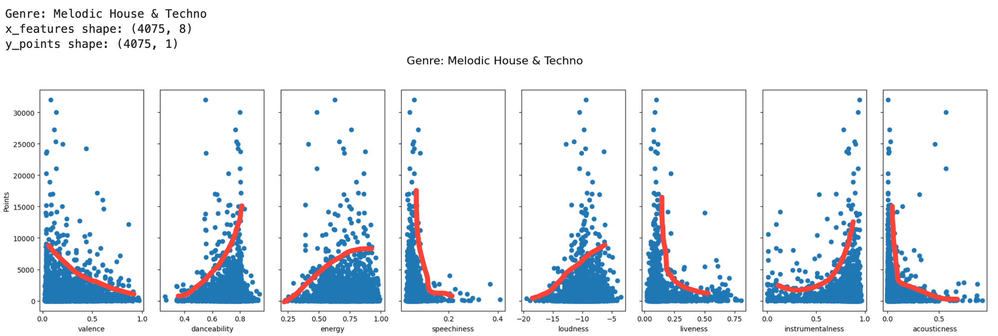
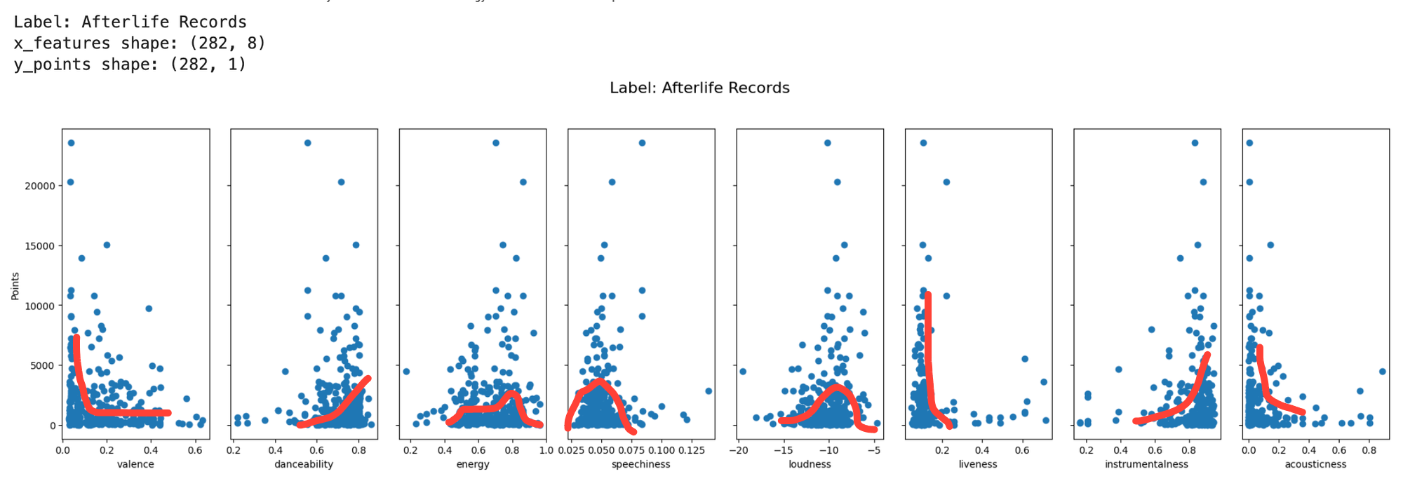
I ran scatterplots for by genre and label for each input feature x against output y points, below are examples for each. The red lines are what I noticed when I first saw them, with the line straight down line for speechniess standing out. To find evidence of the popification of melodic techno, where the music has more lyrics and is barely distinguishable from the mainstage stuff from David Guetta et al, I'll need to unpack that and find micro movements within.

My first thought when I saw the small dataset sizes by the time I got down to the feature and output by label was going to be problematic.

Normalization implementation

Z-Score

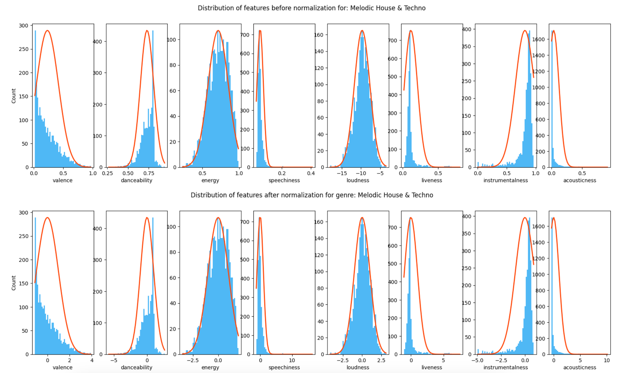
I pucked the way I charted this right out of a deeplearning.ai workbook because I liked it and wanted to see it on some of my data. All of these metrics range from 0.0 to 1.0 so I wasn't really sure what to expect. The skewness of the data was continuing to be the biggest issue to address in the long term. I've just started learning how to handle so, in future project components, I may have a better approach. Still, neat to look at.

Mean normalization

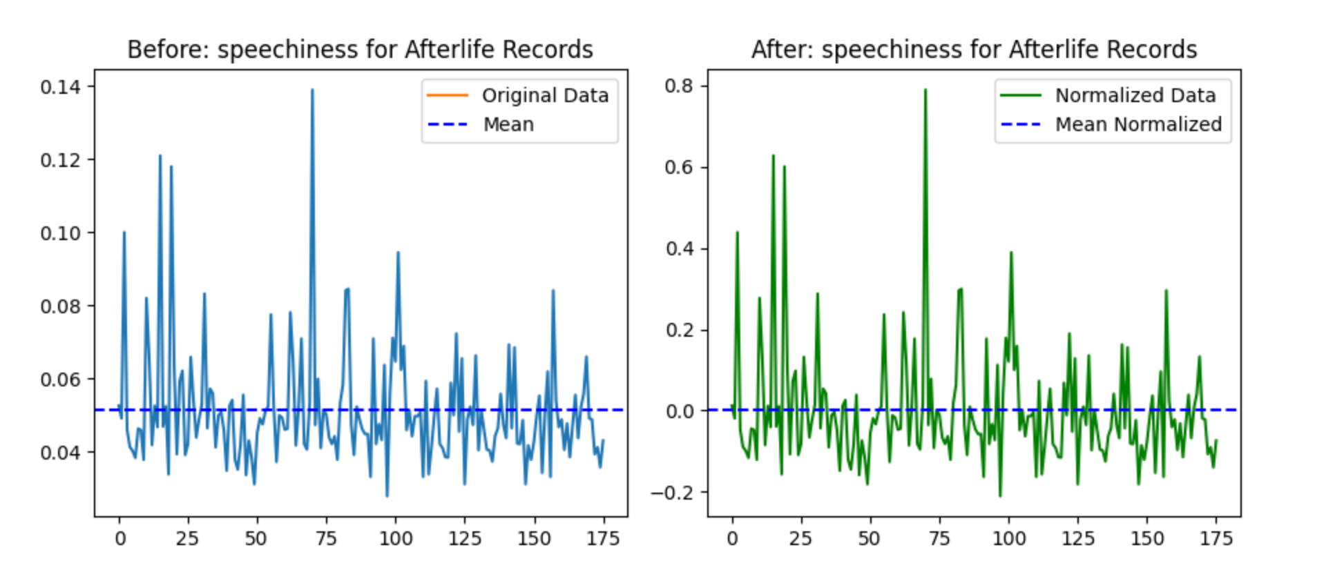
The data gets redistributed to have a mean of zero, so that part worked properly. With the closer-in scale for the x-input, you can see all the bouncing around within the small margin of 0 to .14.

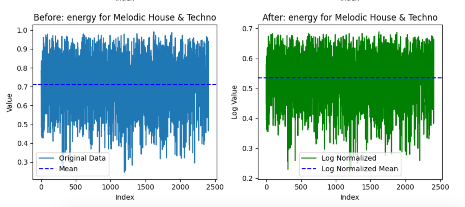
Log normalization

A few signs this one worked as it should have on this data:

• The range gets compressed and goes from 0.3-1.0 to 0.3 to 0.7. Log normalization should compress things and reduce the impact of of both high and low values
• As a result, the mean shifts from 0.7 to around 0.55

Chapter Three

Model execution and output for each normalized data set

def run_all_calculations_genre(train, validate, test):
def run_all_calculations_label(train, validate, test):

This are big ol functions that do the same thing, one for the labels and one for the genres. I'm not going to paste the whole thing here but I'm going to summarize what they do and then highlight a few key parts.

The functions takes train, test, and validate datasets as inputs does different things with different parts:

• Training data: run through the cost, gradient, and gradient descent function
• Cost curves are made for each genre/label and input/output combination and are plotted together.
• Scatter plots with fitted lines are made for train, test, and validate data after gradient descent determines the optimal w and b.
• The Mean Square Error, Root Mean Square Error, Mean Absolute Error, and R Squared are calcuated for each scatter plot combination and placed below the corresponding chart.

This is all happening in one function because I was doing a lot of troubleshooting and didn't want to have to run a bunch of different cells everytime I made an adjustment. It's not super ideal to have all these things tucked in together because it means, for example, they all have to use the same lambda and w values. In the next iterations, once I'm more comfortable with things, I'll either break it up or make the w, b, and lambda parameters function inputs.

Defining subcompoent data for different model execution points

genre_name = subset_genres_dict[genre_id]  # Look up the genre name
        train_genre_mask = (train[:, 7] == genre_id)
        validate_genre_mask = (validate[:, 7] == genre_id)
        test_genre_mask = (test[:, 7] == genre_id)
        
        # Loop through each metric index
        for feature in core_x_features:
            # Apply genre_id filter to points and metric
            x_train = train[train_genre_mask, feature].reshape(-1, 1)
            x_validate = validate[validate_genre_mask, feature].reshape(-1, 1)
            x_test = test[test_genre_mask, feature].reshape(-1, 1)
            
            y_train = train[train_genre_mask, 28]
            y_validate = validate[validate_genre_mask, 28]
            y_test = test[test_genre_mask, 28]

This section creates a mechanism to filter each dataset by the genre_id. Since the train, validate, and shape matrices aren't the same size, I couldn't run the same thing for all three. Technically I might have been able to for validate and test since those are both 20% but, in the moment, decided this was easier to read and follow. I'm able to get the genre_name by looking up the genre_id against that dictionary I showed you earlier.

What cost, gradient, and gradient descent look like in context

cost = single_var_cost_function(x_train, y_train, cost_function_w, cost_function_b, cost_function_lambdar)

tmp_dj_dw, tmp_dj_db = single_var_compute_gradient(x_train, y_train, gradient_w, gradient_b, gradient_lambdar)
            
            # Run gradient descent
            optimal_w, optimal_b, cost_history, w_history = single_var_gradient_descent(x_train, y_train, gradient_w, gradient_b, 
                                                     single_var_cost_function, single_var_compute_gradient, learning_rate, iterations, gradient_lambdar)

            genre_cost_histories[f'{genre_name}-{metric_name}'] = cost_history
            genre_w_histories[f'{genre_name}-{metric_name}'] = w_history

This is where you can see gradient descent taking the cost and gradient functions as inputs so it can produce its output. Each iteration cost j and parameter w is saved and stored in the cost_history and w_history variables so they can be graphed later.

The key thing is: initial cost is run, gradients are established, and then gradient descent is run using them. You want to lower your w and b as much as you can so your cost is as low as it can.

Cost curve graphs

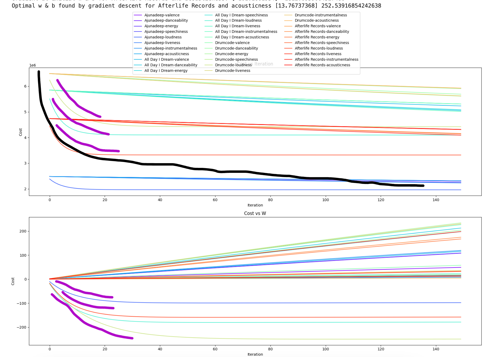
The top graph is cost per iteration, with eqch iteration representing multiple cost calculations that are stored in run_all_calculations_label. The bottom one is cost per parameter w value, which was stored as part of the gradient descent function I showed above.

Aside from having very pretty colors, graphing the different cost outputs for j and w together shows what's going on with cost. The black lines represent what each chart should look like if gradient descent is going well. I've been told by very smart people that there's a small enoough learning rate across a large enough number of iterations that will help the model reach global minimum (the ski resort).

The magenta lines represent where different parts of different lines are doing things that look like so there's something going right at some parts of some lines. I need to do a better job of making each line clearer to make to the legend. While the colors are very pretty and the labels can be identified, it's not easy to identify the specific metric. Those three magenta lines on the top graph are probably the same mtric since they're behaving similarly.

Linear fit with optimized parameters

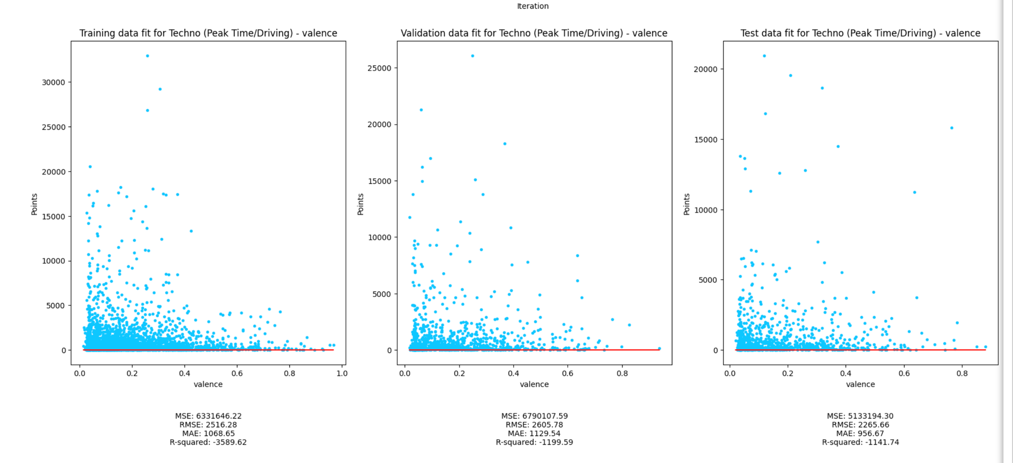
The large negative R Squared means the model fits worse than a horizontal line (lol). A few theories on what's going on:

• Not ideal for linear models: as you've seen from a few different angles, the data doesn't really fit straight lines. If there's a relationship to be had, and I'm not saying there is going to be one, it most likely won't be linear.
• High variance: a model that underfits (which all of the below very much do) is said to have high variance. This means there are large distances between predicted and known values.
  • The inverse problem is high bias, where the line fits too well. You can spot bias by divergences in performance of training versus validate lines. The training line will fit really well because the model has seen that data but doesn't generalize well so when a dataset comes along that it hasn't seen, it doesn;'t do well

Chapter Four

Final thoughts

Overall, I'm satisfied with how part 1 went. I generated a lot of views of the data, which helped me understand what's going on better. There may not have been strong relationships under the first set of conditions, but there's plenty of room to keep looking around.

In the next chunk of work, I'll do polynomial regressions, which allow lines to fit to data that aren't well suited for linear. Remember polynomial math from like high school or something? It's so back, baby. I'll also throw some multi input linear regression at the wall, which is where you can have multiple x inputs for one y output and see if that exposes a relationship.

For the above model, there are a bunch of things I could do. Change w, b, and lambda inputs. Increase or decrease learning rate to change the speed going down the hill.

There's a balancing act I have to strike, though. I want to move into the more advanced things I've learned recently that would help use this data model. Ultimately, I don't want to spend all my time with linear regression since, what I really want to do, is build a music popularity tool that involves some of the large language models out there.