Project Ventoux summit: multilayer neural network with TensorFlow

Summit Supporting Links:

• Github Repository with Jupyter Notebook

• Blog post about my thoughts on this work

General Thoughts

What I've learned, both from smart people telling me in the courses I've been taking and also my own experience, is that creating a deep neural network (mine is 4 layers and they say 5 layers is the threshold for a deep network) has just a ton of tiny little things that need to be controlled for. There are your parameters, the numbers being optimized to create the optimal loss value. There are the hyper parameters that influence the parameters, like number of layers, neurons, lambda value, optimization approach. Do you run all neurons or every time or try dropout to train the model to not be reliant on any given value coming in?

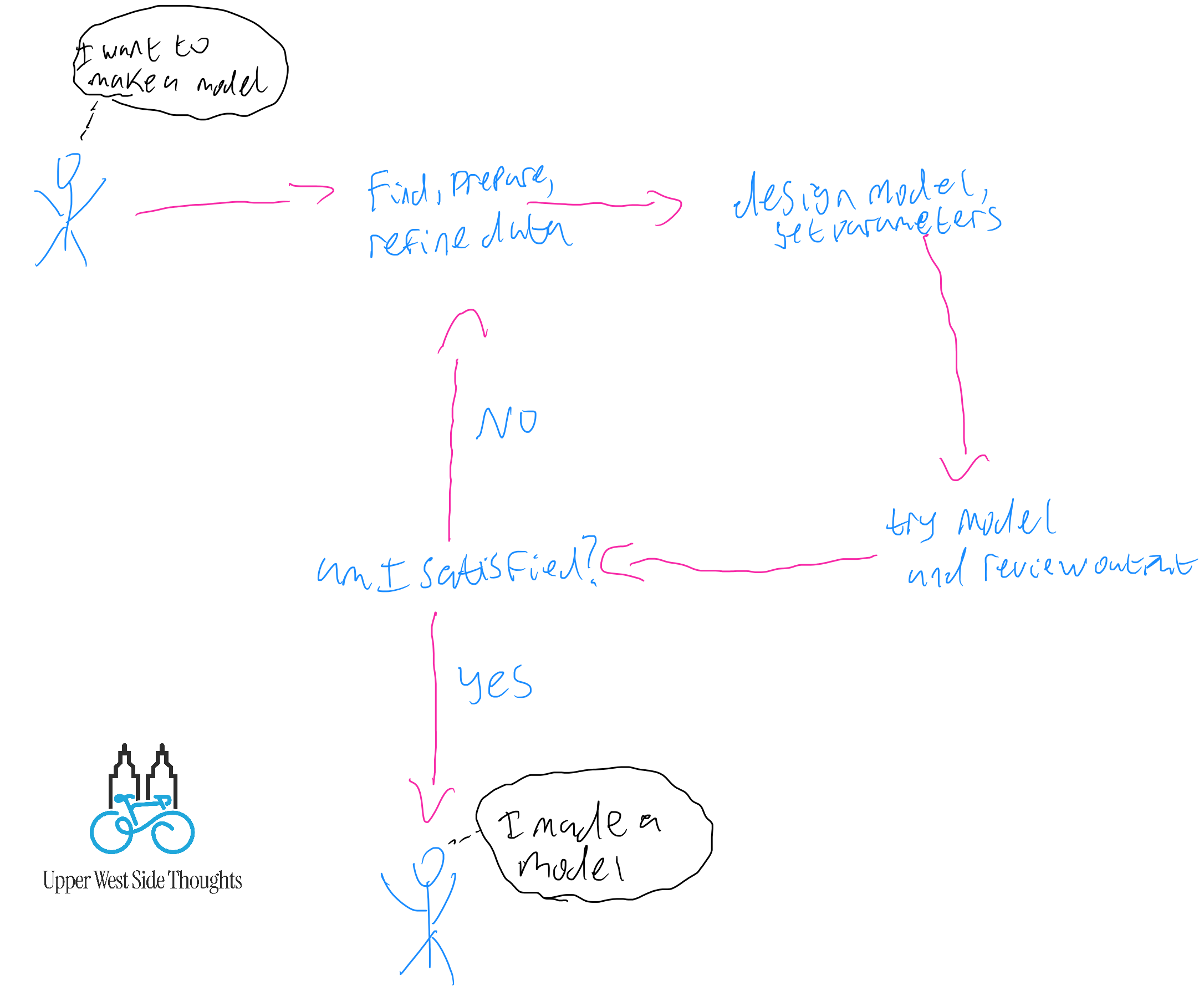
This is what the process ends up being. It's not uncommon to go around a bunch of times before you decide you're satisfied. Most models (including mine) fail or underperform or otherwise behave in ways you don't like the first time. You want to take your time and get it right, even if it means changing the model entirely. You're going to do a whole lot of messing around and then a whole lot of finding out.

All of this brings and end to Project Ventoux, with Project Dolly Shield coming to the vanguard. This will let me go back to the very beginning, with a much larger set of data, and a whole lot of new skills, to create a much more sophisticated outcome. In additional, I'm starting on natural language processing and am looking for approaches to fine tuning a large language model. I also have a bunch of Midi and WAV music files and want to see if I can do something with models from organizations like Magenta. Head on over to Dolly Shield to learn more about what's on my mind.

Initial Network Plans

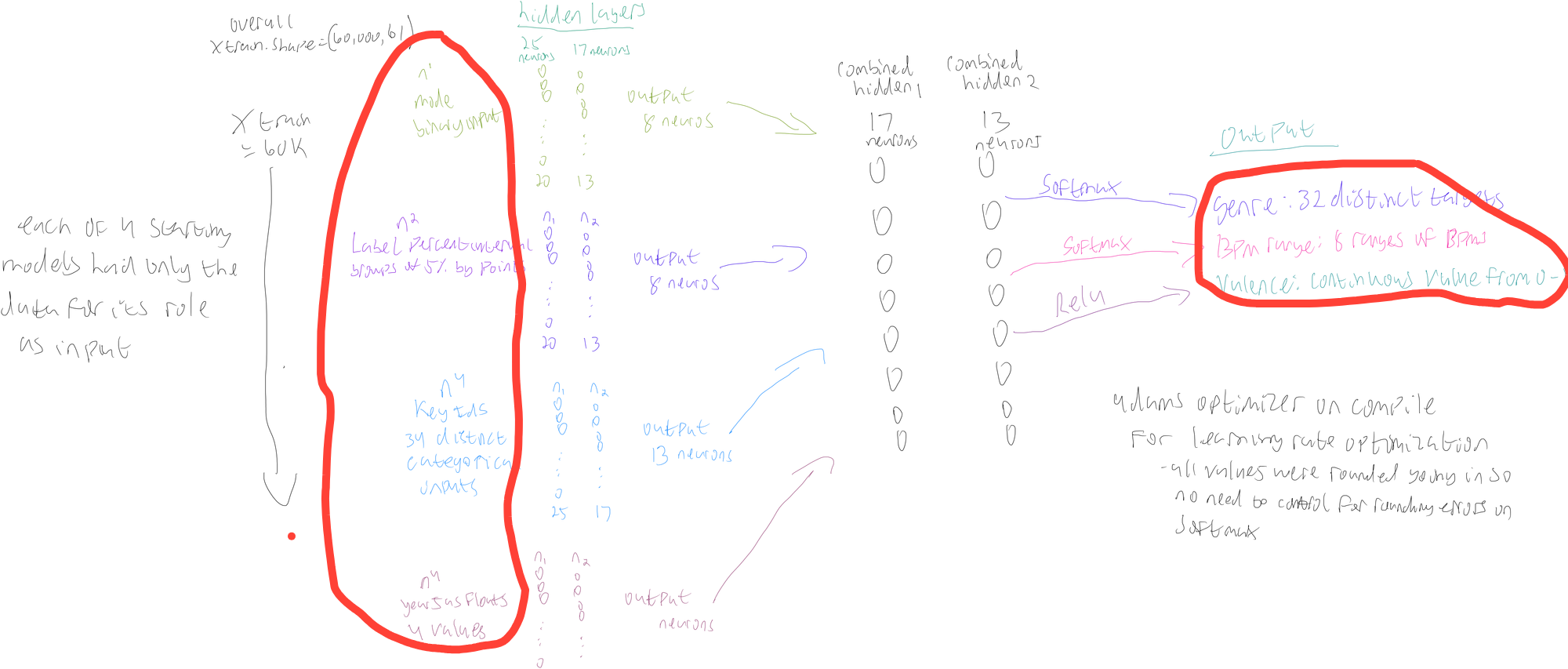
On this drawing below, I've circled two parts in red: the X-input features I knew I wanted to start with and the three output features I knew I wanted to end with. Everything in between I iterated through as I implemented best practices.

Each X-train input and Y-output target set had around 60,000 rows of data.

You can review the "importing bigger files and creating subset I want for neural network" section of the linked notebook to see all the work I see to create the below feature groupings, which I briefly describe.

• Categorical features:
  • X-train input: Label Percent Intervals. grouped label IDs into 5% groupings, based on Beatport Points. The top 5% of labels by points are together, then the next 5%, etc. This is because they were 77,000+ distinct label IDs, which would have cause matrix explosion on encoding if I wanted to maintain its inherently categorical quality.
  • X-train input: Key IDs. Beatport only has 34 IDs for the music note keys that can be assigned to a song, with each song having one ID. The same ID can be assigned to multiple songs.
  • X-train input: year, represented as a float. This is the year a song was released, so 2019 is 2019.0. I culled the list down to the four years I had substantial data for, which is 2019-2023.
  • Y-train output: genre. Beatport has 32 predefined genres and the output is an ID that links back to one.
    • Uses the Softmax activation function with the CategoricalCrossentropy losss function since it's a one hot encoded categorical output, where each genre is a category
  • Y-train output: BPM range. Beats Per Minute define the tempo of a track and I grouped the BPMs into different ranges, based on what made sense. For instance: 0-60 are all together since there aren't many songs down there but 120-130 is one group and 131-140 is another
    • Also uses the Softmax activation function with the CategoricalCrossentropy loss function since it's a one hot encoded categorical output, where each BPm range is a category. SparseCategoricalCrossentropy is an option when the output isn't one hot encoded.
• Numerical features:
  • Y-train output: valence. A continuous numerical output that ranges from 0 to 1
    • Uses the Sigmoid activation function with the MeanSquaredError() loss function since this is an output that can only be positive and between 0 and 1. Softmax activation is for categorical outputs.

This shows the chunk of code that creates the year, label_percent_interval, and bpm_range

filtered_df = toptracks_bpmeta_matrix_df.loc[
     (toptracks_bpmeta_matrix_df['release_year'] >= 2019.0) & 
    (toptracks_bpmeta_matrix_df['release_year'] <= 2024.0)
 ].copy()

 # grouping labels in % intervals based on points 
 filtered_df.loc[:, 'label_percent_interval'] = tian.qcut(filtered_df['points'], 20, labels=False) / 20.0

 #bpm range 
 bpm_range = [0, 60, 100, 110, 120, 130, 140, 150, 300]
 filtered_df.loc[:, 'bpm_group'] = tian.cut(filtered_df['bpm'], bpm_range, right=False)

Encoding Data and Creating Train, Validate, and Test Sets

The next two blocks of code cover large chunks of transformation process that took me from a baseline matrix to datasets that can be used in the model further down.

This required a lot of troubleshooting as I traced different array mismatch errors I encountered when I first executed the model. I have a lot of logging of array sizes because I need to ensure each component had similar sizes. A common error I ran into early was something like "model expecting a X by 4 array but you gave it in X by 3 array."

Input and Target Arrays

two_layer_inputs = [1, 2, 6, 7]
inputs = pogi_soar_matrix[:, two_layer_inputs]

# genre ID, bpm_group, valence as targets
two_layer_targets = [3, 5, 8]
targets = pogi_soar_matrix[:, two_layer_targets]

# get unique categories 
year_uniques = set(inputs[:, 0])
label_percent_uniques = set(inputs[:, 1])
key_uniques = set(inputs[:, 2])
mode_uniques = set(inputs[:, 3])

print(f'input years: {year_uniques}')
print(f'input label %: {label_percent_uniques}')
print(f'input keys: {key_uniques}')
print(f'input modes: {mode_uniques}')

genre_uniques = set(targets[:, 0])
bpm_uniques = set(targets[:, 1])
valence_uniques = list(set(targets[:, 2]))

print(f'target genres: {genre_uniques}')
print(f'target bpms: {bpm_uniques}')
print(f'target valence (example): {valence_uniques[:10]}')

Encoding and Splitting

Categorical transformation was done with OneHotEncoding so that a single column with potentially 30 values became 31 columns, each a binary 0/1 value to say if it applies or not. For something like genre, where there's only one value per song, it would be 1 in one column and 0's in the rest.

This resulted in a 61 column array: 20 for label percent group, 34 for genre, 4 four year, and the rest for mode. "What all that printing results in" in the toggle below the code shows how the different subsets become transformed components.

def quantile_transform_data(data):
    transformer = QuantileTransformer(output_distribution='normal')
    return transformer.fit_transform(data.reshape(-1, 1)).flatten()

# valence quantile transform
valence_index = two_layer_targets.index(8)
valence_data = targets[:, valence_index]
valence_transformed = quantile_transform_data(valence_data)
targets[:, valence_index] = valence_transformed

# transformers for categorical and numerical data
categorical_transformer = OneHotEncoder(sparse_output=False)
numerical_transformer = MinMaxScaler()

input_preprocessor = ColumnTransformer(
    transformers=[
        ('categorical', categorical_transformer, [0, 1, 2, 3])  
    ]
)

target_preprocessor = ColumnTransformer(
    transformers=[
        ('categorical', categorical_transformer, [0, 1]), 
        ('numerical', numerical_transformer, [2])       
    ]
)

# check original shape
print("Original matrix shape:", pogi_soar_matrix.shape)

# transform inputs and outputs
inputs_transformed = input_preprocessor.fit_transform(inputs)
print("Transformed inputs shape:", inputs_transformed.shape)

targets_transformed = target_preprocessor.fit_transform(targets)
print("Transformed targets shape:", targets_transformed.shape)

# train/validate/test split
X_train, X_temp, y_train, y_temp = train_test_split(inputs_transformed, targets_transformed, test_size=0.40, random_state=1)
X_cv, X_test, y_cv, y_test = train_test_split(X_temp, y_temp, test_size=0.50, random_state=1)

# post-split check
print("X_train.shape:", X_train.shape)
print("y_train.shape:", y_train.shape)
print("X_cv.shape:", X_cv.shape)
print("y_cv.shape:", y_cv.shape)
print("X_test.shape:", X_test.shape)
print("y_test.shape:", y_test.shape)

# train, validate, and test input sets based on where each feature lies as columns in the 61 columns of encoded matrix
X_train_year = X_train[:, :4]  
X_train_label = X_train[:, 4:24]  
X_train_key = X_train[:, 24:58] 
X_train_mode = X_train[:, 58:] 

print("X_train_year:", X_train_year.shape)
print("X_train_label:", X_train_label.shape)
print("X_train_key:", X_train_key.shape)
print("X_train_mode:", X_train_mode.shape)

X_cv_year = X_cv[:, :4]
X_cv_label = X_cv[:, 4:24]
X_cv_key = X_cv[:, 24:58]
X_cv_mode = X_cv[:, 58:]

print("X_cv_year:", X_cv_year.shape)
print("X_cv_label:", X_cv_label.shape)
print("X_cv_key:", X_cv_key.shape)
print("X_cv_mode:", X_cv_mode.shape)

X_test_year = X_test[:, :4]
X_test_label = X_test[:, 4:24]
X_test_key = X_test[:, 24:58]
X_test_mode = X_test[:, 58:]
print("X_test_year:", X_test_year.shape)
print("X_test_label:", X_test_label.shape)
print("X_test_key:", X_test_key.shape)
print("X_test_mode:", X_test_mode.shape)

# train, validate, and test output sets based on where each feature lies as columns in the 61 columns of encoded matrix
y_train_genre = y_train[:, :len(genre_uniques)]
y_train_bpm = y_train[:, len(genre_uniques):(len(genre_uniques) + len(bpm_uniques))]
y_train_valence = y_train[:, -1]  # Last column for valence

print("y_train_genre:", y_train_genre.shape)
print("y_train_bpm:", y_train_bpm.shape)
print("y_train_valence:", y_train_valence.shape)

y_cv_genre = y_cv[:, :len(genre_uniques)]
y_cv_bpm = y_cv[:, len(genre_uniques):(len(genre_uniques) + len(bpm_uniques))]
y_cv_valence = y_cv[:, -1]

y_test_genre = y_test[:, :len(genre_uniques)]
y_test_bpm = y_test[:, len(genre_uniques):(len(genre_uniques) + len(bpm_uniques))]
y_test_valence = y_test[:, -1]

print("y_cv_genre:", y_cv_genre.shape)
print("y_cv_bpm:", y_cv_bpm.shape)
print("y_cv_valence:", y_cv_valence.shape)

print("y_test_genre:", y_test_genre.shape)
print("y_test_bpm:", y_test_bpm.shape)
print("y_test_valence:", y_test_valence.shape)

TensorFlow Network Definition

Subnetwork Definition

This is the function I created to define the sub-network that each feature goes through independently:

def pogi_prep():
    soigneur = Sequential([
        Input(shape=(1,)),
        Dense(25, activation='relu', kernel_regularizer=l2(0.01)),
        Dense(17, activation='relu', kernel_regularizer=l2(0.01)),
    ])
    return soigneur

label_input = Input(shape=(1,), name='label_percent_interval')
key_input = Input(shape=(1,), name='key')
mode_input = Input(shape=(1,), name='mode')
release_year_input = Input(shape=(1,), name='release_year')

Main Network Definition

def pogi_slay():
    label_input = Input(shape=(20,), name='label_percent_interval')  
    key_input = Input(shape=(34,), name='key')  
    mode_input = Input(shape=(3,), name='mode')  
    release_year_input = Input(shape=(4,), name='release_year')  # One-hot encoded with 4 categories

    # uae pogi_prep to create subnetwork for each input
    label_features = pogi_prep(20)(label_input)
    key_features = pogi_prep(34)(key_input)
    mode_features = pogi_prep(3)(mode_input)
    release_year_features = pogi_prep(4)(release_year_input)

    # string together the different features for use in combined model
    false_flat = Concatenate()([label_features, key_features, mode_features, release_year_features])

    # combined model hidden layers
    dolly_hidden = Dense(13, activation='relu', kernel_regularizer=l2(0.1))(false_flat)
    pogi_hidden = Dense(10, activation='relu', kernel_regularizer=l2(0.1))(dolly_hidden)

    # final outputs

    #32 genres
    genre_slay = Dense(32, activation='softmax', name='genre_id')(pogi_hidden)  
    
    # 8 BPM groups created
    bpm_4tofloor = Dense(8, activation='softmax', name='bpm_group')(pogi_hidden) 

    #single output ranging from 0 to 1 on continuous scale
    valence_smile = Dense(1, activation='sigmoid', name='valence')(pogi_hidden)  # Regression-like output for valence

    # defines final model
    pogi_wheels = Model(inputs=[label_input, key_input, mode_input, release_year_input], 
                        outputs=[genre_slay, bpm_4tofloor, valence_smile])

    return pogi_wheels

Compile Definition

I continue to use the Adams Optimizer for the learning rate. When you're working with data that's vulnerable to the round off error and you're working with categorical data (maybe others? I still need to learn), you can set the final layer of the network to have a linear activation function. In the compile you add a "from_logit=True" on the loss component and that tells the adams optimizer to treat the linear activation as a softmax activation while also handling the round off error.

The compile also includes a metrics section. This logs the desired data, which I can then use later in evaluation and general setup.

#executes and compiles final model
ventoux_summit = pogi_slay()

ventoux_summit.compile(
    #adamds optimizer alllows for automatic adjustments of learning rate in gradient descent instead of having to try a bunch of options
    optimizer=Adam(learning_rate=0.001),
    loss={
        'genre_id': CategoricalCrossentropy(),  
        'bpm_group': CategoricalCrossentropy(),  
        'valence': MeanSquaredError() 
    },
    metrics={
        'genre_id': ['accuracy', Precision(), Recall()],
        'bpm_group': ['accuracy', Precision(), Recall()],
        'valence': 'mean_squared_error'
    }
)

Model Execution and Evaluation

Model Fitting

The pogi_monitoring field is a TensorBoard function that points data generated from the model to a file directory where that data can be stored. In the summit.fit() execution, the callbacks=[pogi_monitoring] component allows for data to be sent to TensorBoard for realtime monitoring.

The CodePen dashboard below the code shows some of the charts generated during model execution. The charts show generally healthy performance for training. The loss curve for the training data has the natural curve that I had to hand draw before. In a future setup, I'll wire the setup to point to cloud infrastructure for an always-on setup.

pogi_stem = f'{bucket_file_base}/silent_ascent_files/pogi_logs'
pogi_logger = f'{pogi_stem}/{datetime.datetime.now().strftime("%Y%m%d-%H%M%S")}-ventoux_summit'

pogi_monitoring = TensorBoard(log_dir=pogi_logger, histogram_freq=1)

#fitting
pogi_soar = ventoux_summit.fit(
    [X_train_label, X_train_key, X_train_mode, X_train_year], 
    {'genre_id': y_train_genre, 'bpm_group': y_train_bpm, 'valence': y_train_valence}, 
    epochs=10, 
    batch_size=100,
     validation_data=(
     [X_cv_label, X_cv_key, X_cv_mode, X_cv_year], 
     {'genre_id': y_cv_genre, 'bpm_group': y_cv_bpm, 'valence': y_cv_valence}
        ),
    callbacks=[pogi_monitoring]
    )

CodePen Dashboard of TensorBoard Monitoring

Prediction and Evaluation

predictions = ventoux_summit.predict([X_test_label, X_test_key, X_test_mode, X_test_year])

ventoux_evaluation = ventoux_summit.evaluate(
    [X_test_label, X_test_key, X_test_mode, X_test_year], 
    {'genre_id': y_test_genre, 'bpm_group': y_test_bpm, 'valence': y_test_valence}
)

Confusion Matrices for Genre ID and BPM Group

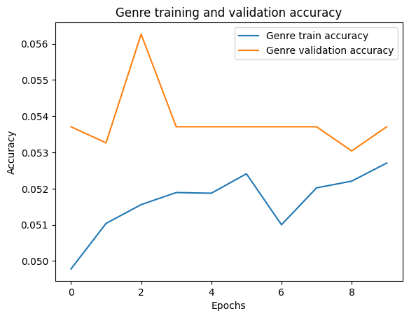
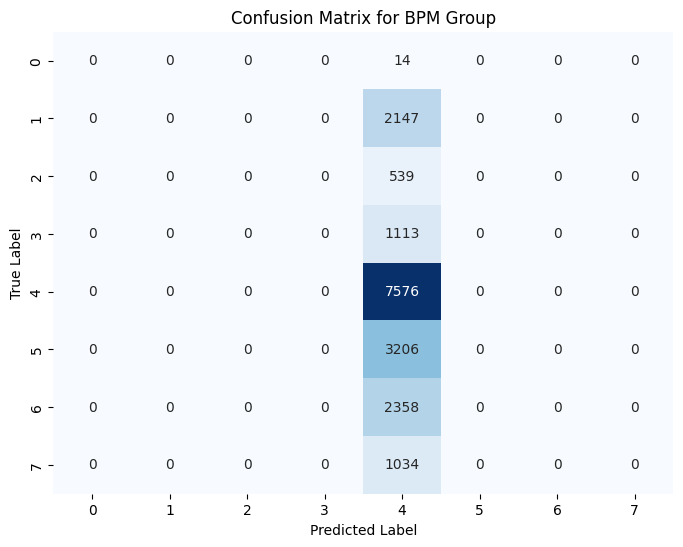
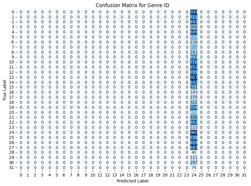
These are fun charts. A confusion matrix shows what the model predicted along the x-axis versus what should have been predicted along the y-axis. As you can see, my model is only predicting one genre or BPM group. This indicates some sort of something going wrong in the matrix creation/encoding process. Something in the data is causing it to only way to predict one outcome.

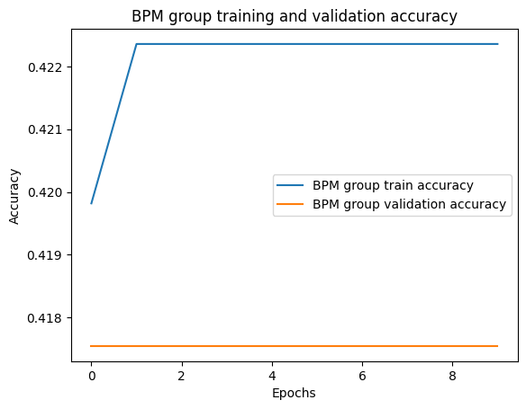
Model Accuracy for Genre ID and BPM Group

The BPM group accuracy appears to be a happy accident that's related to the above. Label 4 is 110-120 BPM. The default BPM when you go to make a song, if you change nothing, is BPM. Most songs live in the 115-125 range and, next time, I would rejigger these ranges to better show that.